14  Introduction to Binomial Tree Model

The binomial tree model is a discrete-time framework used to price derivative securities. It is widely used in financial engineering for valuing options and other contingent claims. This model is particularly useful because it provides an intuitive approach to pricing and allows for easy incorporation of various features such as early exercise in American options.

14.1 Basics of the Binomial Tree Model

The binomial tree model is based on the assumption that, over a small time step, the price of an underlying asset can move up or down by a certain factor. The model is constructed iteratively to estimate the fair value of derivatives such as options.

An \(n\) period binomial tree model can be described as follows:

1. There are \(n+1\) time points with \(t=0, \Delta t, 2 \Delta t, ..., n\Delta t\), where \(\Delta t\) is the time step.

2. At each time point \(t\), the price of the underlying asset either goes up by a factor \(u_t>1\) with probability \(p_t\in(0,1)\) or goes down by a factor \(d_t<1\) with probability \(1-p_t\).

3. Given an initial stock price \(S_0\), the price of the underlying asset evolves as:

\[ S_{t+\Delta t} = S_t \times u_t \quad \text{(up move)} \] or \[ S_{t+\Delta t} = S_t \times d_t \quad \text{(down move)} \]

4. The absence of arbitrage ensures the model can be solved using risk-neutral valuation, where the risk-neutral probability of an up move is:

\[ p_t = \frac{e^{r_t \Delta t} - d_t}{u_t - d_t} \]

where $ r_t $ is the risk-free rate from \(t\) to \(t+\Delta t\).

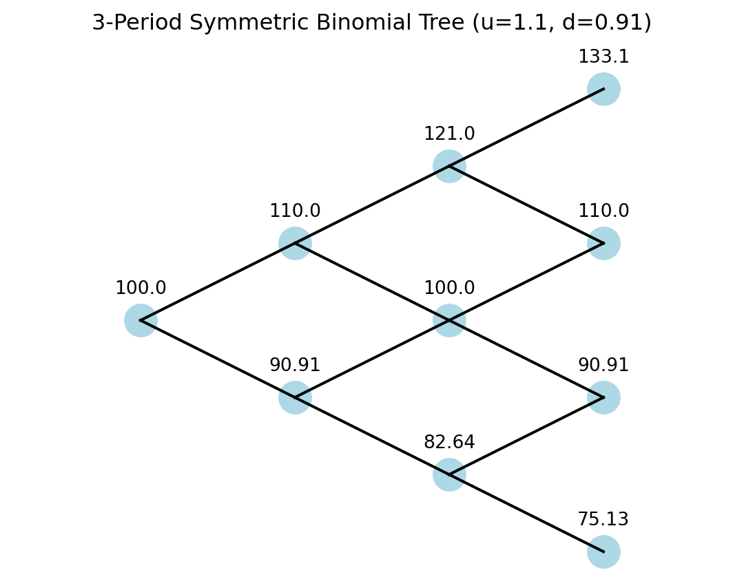
Example: Three-Period Recombining Binomial Tree

This is an example of a three-period recombining binomial tree: \(n=3\), \(u=1.1\), \(d=1/u\), \(\Delta t=1\):

import plotly.graph_objects as go

def plot_symmetric_binomial_tree(S0=100, u=1.1):
    d = 1 / u  # Down factor
    periods = 3  # Number of periods

    # Define nodes with symmetric positioning
    nodes = {}
    for t in range(periods + 1):
        for j in range(t + 1):
            x = t  # Time step on x-axis
            y = 2 * j - t  # Centered y-axis positioning for symmetry
            nodes[(x, y)] = round(S0 * (u ** j) * (d ** (t - j)), 2)

    # Define edges
    edges = []
    for t in range(periods):
        for j in range(t + 1):
            x = t
            y = 2 * j - t
            edges.append(((x, y), (x + 1, y + 1)))  # Up move
            edges.append(((x, y), (x + 1, y - 1)))  # Down move

    fig = go.Figure()

    # Add edges to the plot
    for edge in edges:
        x_coords = [edge[0][0], edge[1][0]]
        y_coords = [edge[0][1], edge[1][1]]
        fig.add_trace(go.Scatter(x=x_coords, y=y_coords, mode='lines', line=dict(color='black'), showlegend=False))

    # Add nodes to the plot
    x_vals = [key[0] for key in nodes.keys()]
    y_vals = [key[1] for key in nodes.keys()]
    labels = [str(nodes[key]) for key in nodes.keys()]

    fig.add_trace(go.Scatter(
        x=x_vals, y=y_vals, mode='markers+text',
        marker=dict(size=20, color='lightblue'),
        text=labels, textposition="top center",
        showlegend=False
    ))

    fig.update_layout(
        title="3-Period Symmetric Binomial Tree (u=1.1, d=1/u)",
        xaxis=dict(showgrid=False, zeroline=False, showticklabels=False),
        yaxis=dict(showgrid=False, zeroline=False, showticklabels=False),
        plot_bgcolor='white',
        width=700,
        height=500
    )

    fig.show()

plot_symmetric_binomial_tree()

import matplotlib.pyplot as plt

def plot_symmetric_binomial_tree(S0=100, u=1.1, vertical_scale=0.5, title_pad=20):
    """
    Plots a 3-period symmetric binomial tree using Matplotlib,
    with options to compress the vertical spacing and add space between the title and the plot.

    :param S0: initial stock price
    :param u: up factor
    :param vertical_scale: compresses or expands the vertical spacing
    :param title_pad: extra spacing between the title and the tree (in points)
    """
    d = 1 / u  # Down factor
    periods = 3  # Number of periods

    # Define nodes with symmetric positioning
    nodes = {}
    for t in range(periods + 1):
        for j in range(t + 1):
            x = t
            y = vertical_scale * (2 * j - t)  # scale the vertical distance
            nodes[(x, y)] = round(S0 * (u**j) * (d**(t - j)), 2)

    # Define edges
    edges = []
    for t in range(periods):
        for j in range(t + 1):
            x = t
            y = vertical_scale * (2 * j - t)
            # Up move
            edges.append(((x, y), (x + 1, y + vertical_scale)))
            # Down move
            edges.append(((x, y), (x + 1, y - vertical_scale)))

    # Create a Matplotlib figure
    fig, ax = plt.subplots(figsize=(7, 5))

    # Plot edges
    for edge in edges:
        x_coords = [edge[0][0], edge[1][0]]
        y_coords = [edge[0][1], edge[1][1]]
        ax.plot(x_coords, y_coords, color='black')

    # Plot nodes
    x_vals = [k[0] for k in nodes.keys()]
    y_vals = [k[1] for k in nodes.keys()]
    labels = [str(nodes[k]) for k in nodes.keys()]
    ax.scatter(x_vals, y_vals, s=300, color='lightblue')

    # Add text labels above each node
    for x, y, label in zip(x_vals, y_vals, labels):
        ax.text(x, y + 0.3 * vertical_scale, label, ha='center', va='bottom')

    # Title with extra spacing set by 'pad'
    ax.set_title(
        f"3-Period Symmetric Binomial Tree (u={u}, d={round(d,2)})",
        pad=title_pad
    )

    # Style the plot
    ax.axis("equal")
    ax.axis("off")

    plt.show()

# Example usage: extra spacing of 20 points between the caption and the tree
plot_symmetric_binomial_tree(vertical_scale=0.5, title_pad=20)

14.2 Approximation of Continuous Stochastic Processes

A binomial tree is a discrete-time stochastic process with two possible outcomes at each time step. In its simplest form, at every step the process moves either up or down by a fixed factor or amount, with specified probabilities. This construction can be used to approximate almost any continuous stochastic processes. The main idea is as follows:

1. Discrete Steps:

   In a binomial tree, time is divided into small increments (say, \(\Delta t\)). At each time step, the process moves up by a factor \(u\) or down by a factor \(d\). This is analogous to a random walk where at each step you move one unit to the right or left.

2. Probabilities and Expected Change:

   By choosing the probabilities (say \(p\) for an up move and \(1-p\) for a down move) appropriately, you can control the drift and variance of the process. For a symmetric random walk, you might set \(p = 0.5\). More generally, one can adjust these parameters so that, over many steps, the binomial model matches the first two moments (mean and variance) of the random walk you want to approximate.

3. Convergence to a Continuous Process:

   As you make the time steps smaller (i.e., \(\Delta t \to 0\)) and choose \(u\) and \(d\) appropriately (for example, \(u = e^{\sigma\sqrt{\Delta t}}\) and \(d = e^{-\sigma\sqrt{\Delta t}}\) for volatility \(\sigma\)), the binomial process converges in distribution to a continuous-time process, such as Brownian motion (or a geometric Brownian motion if you’re modeling stock prices).

4. Example:

   Suppose you have a simple random walk starting at 0. At each time step:

   • With probability \(0.5\), add 1 (up move).
   • With probability \(0.5\), subtract 1 (down move).

   This is a binomial tree where the position after \(n\) steps is given by: \[ X_n = X_0 + (\text{number of up moves}) - (\text{number of down moves}). \] As \(n\) grows, by the Central Limit Theorem, the distribution of \(X_n\) becomes approximately normal, just like a random walk with Gaussian increments.

5. Application in Finance:

   In financial modeling, the binomial tree is used to approximate the price evolution of an asset. The tree method provides a simple numerical technique to value options and other derivatives by stepping through the possible future asset prices and then discounting back to the present.

In summary, the binomial tree model can approximate a continuous stochastic process by discretizing time into small intervals with two possible outcomes at each step. With the right choice of parameters and as the step size decreases, the binomial process can approximate well the behavior of the continuous stochastic process, while keeping the numerical valuation of simple.

14.3 A Generalized \(n\)-Period Tree

We can generalize the above basic binomial tree to a more general one where each node at any time \(t\) can have a variable number of branches and the branching pattern can vary across both time steps and nodes. This flexible structure can be useful for pricing more complex derivative securities.

Definition of a Generalized \(n\)-period tree

1. Tree Structure

We define the tree as a directed graph \(T = (N, E)\), where:

• \(N\) is the set of nodes.
• \(E \subseteq N \times N\) is the set of edges, representing transitions between nodes across periods.

Each node is indexed by:

\[ N_{t,i}, \quad t = 0, 1, \dots, n, \quad i = 1, \dots, |N_t| \]

where:

• \(t\) represents the time point,
• \(i\) represents the node index at time \(t\),
• \(|N_t|\) denotes the number of nodes at time \(t\).

---

2. Variable Branching

Each node \(N_{t,i}\) has \(B_{t,i}\) branches, which represents the number of children (next-period nodes) it connects to. The total number of nodes at time \(t+1\) is then:

\[ |N_{t+1}| = \sum_{i=1}^{|N_t|} B_{t,i} \]

Each edge represents a transition probability \(P_{t,i,j}\) from node \(N_{t,i}\) at time \(t\) to node \(N_{t+1, j}\) at time \(t+1\), satisfying:

\[ \sum_{j=1}^{B_{t,i}} P_{t,i,j} = 1, \quad \forall i, t \]

where \(P_{t,i,j}\) is the probability of transitioning from \(N_{t,i}\) to \(N_{t+1,j}\).

---

3. Node Values and Transition Rule

Each node has a value \(S_{t,i}\), which can represent an evolving variable (e.g., stock price, state variable). The value transition function is defined as:

\[ S_{t+1,j} = f(S_{t,i}, a_{t,i,j}) \]

where:

• \(S_{t,i}\) is the value at node \(N_{t,i}\),
• \(a_{t,i,j}\) is a transition factor specific to the branch from \(N_{t,i}\) to \(N_{t+1,j}\),
• \(f\) is a value update function, often modeled as: \[ S_{t+1,j} = S_{t,i} \times a_{t,i,j} \]

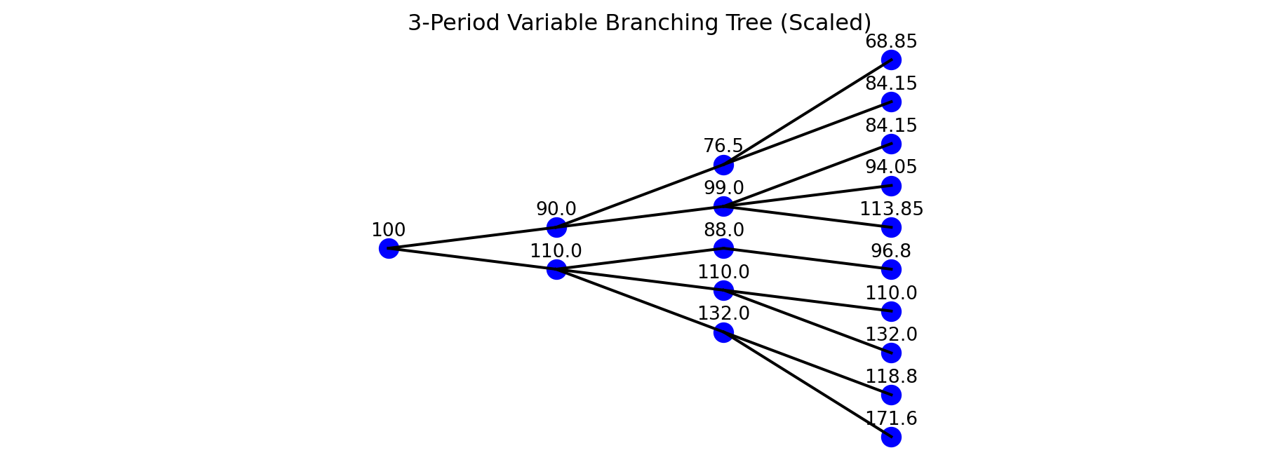
Example: Consider a 3-period tree with variable branching:

• Period 0: 1 node (\(B_{0,1} = 2\))
• Period 1: 2 nodes, each with different branching (\(B_{1,1} = 3, B_{1,2} = 2\))
• Period 2: 5 nodes, each branching further (\(B_{2,1} = 2, B_{2,2} = 2, B_{2,3} = 1, B_{2,4} = 3, B_{2,5} = 2\)).

The node count evolves as:

\[ |N_1| = B_{0,1} = 2, \quad |N_2| = B_{1,1} + B_{1,2} = 3 + 2 = 5, \quad |N_3| = 2 + 2 + 1 + 3 + 2 = 10 \]

Thus, a generalized tree dynamically adjusts the branching structure.

Special Cases

• Binomial Tree (\(B_{t,i} = 2\)): Each node has exactly two branches, leading to an up/down model.
• Trinomial Tree (\(B_{t,i} = 3\)): Each node has three possible transitions (e.g., up, middle, down).
• Adaptive Trees: \(B_{t,i}\) can depend on volatility or other dynamic parameters.

A Graphical Illustration of a Generalized 3-Period Tree

Here is a 3-period example with variable branching:

import plotly.graph_objects as go
from collections import defaultdict

def plot_variable_branching_tree_symmetric():
    # 1. Build tree nodes/edges
    nodes = {(0, 0): 100}  # Root node at time t=0, index=0 => value=100
    edges = []

    # next_index[t] tracks how many nodes have been created at period t so far
    next_index = defaultdict(int)
    next_index[0] = 1  # We have 1 node at t=0

    # transitions[(t, i)] = list of factors for each branch out of node (t, i)
    transitions = {
        (0, 0): [1.1, 0.9],       # At t=0, i=0 => 2 branches
        (1, 0): [1.2, 1.0, 0.8],  # At t=1, i=0 => 3 branches
        (1, 1): [1.1, 0.85],      # At t=1, i=1 => 2 branches
        (2, 0): [1.3, 0.9],       # At t=2, i=0 => 2 branches
        (2, 1): [1.2, 1.0],       # At t=2, i=1 => 2 branches
        (2, 2): [1.1],            # At t=2, i=2 => 1 branch
        (2, 3): [1.15, 0.95, 0.85], # t=2, i=3 => 3 branches
        (2, 4): [1.1, 0.9]        # t=2, i=4 => 2 branches
    }

    # Create nodes/edges
    for (t, i), factors in transitions.items():
        base_value = nodes[(t, i)]
        for factor in factors:
            child_t = t + 1
            child_i = next_index[child_t]
            next_index[child_t] += 1

            child_value = round(base_value * factor, 2)
            nodes[(child_t, child_i)] = child_value

            edges.append(((t, i), (child_t, child_i)))

    # 2. Count how many nodes per period => assign symmetrical y-coordinates
    nodes_in_period = defaultdict(list)
    for (t, i), val in nodes.items():
        nodes_in_period[t].append(i)

    # For each period t, sort node indexes, then map them to symmetrical positions around 0
    coords = {}  # coords[(t, i)] = y_position
    for t in sorted(nodes_in_period.keys()):
        node_list = sorted(nodes_in_period[t])
        count = len(node_list)

        # We'll assign positions from 0..(count-1), then shift so center is 0
        for idx, node_i in enumerate(node_list):
            # E.g., if count=5, positions -> 0,1,2,3,4 => shift by -2 => -2,-1,0,1,2
            shift = -(count - 1) / 2
            y = idx + shift
            coords[(t, node_i)] = y

    # 3. Build the plot
    fig = go.Figure()

    # Add edges
    for ((t1, i1), (t2, i2)) in edges:
        x_coords = [t1, t2]
        y_coords = [coords[(t1, i1)], coords[(t2, i2)]]
        fig.add_trace(go.Scatter(
            x=x_coords,
            y=y_coords,
            mode='lines',
            line=dict(color='black'),
            showlegend=False
        ))

    # Add nodes (markers+text)
    for (t, i), val in nodes.items():
        fig.add_trace(go.Scatter(
            x=[t],
            y=[coords[(t, i)]],
            mode='markers+text',
            marker=dict(size=10, color='blue'),
            text=[str(val)],
            textposition='top center',
            showlegend=False
        ))

    fig.update_layout(
        title="3-Period Variable Branching Tree (Symmetric Layout)",
        xaxis=dict(showgrid=False, zeroline=False, showticklabels=False),
        yaxis=dict(showgrid=False, zeroline=False, showticklabels=False),
        width=900,
        height=600,
        plot_bgcolor='white'
    )

    fig.show()

# Call the plotting function
plot_variable_branching_tree_symmetric()

import matplotlib.pyplot as plt
from collections import defaultdict

def plot_variable_branching_tree_scaled(vertical_scale=0.5, horizontal_scale=2.0):
    """
    Plots a 3-period variable branching tree in a narrower vertical 
    layout and a longer horizontal layout.

    :param vertical_scale: Factor (<1 = narrower, >1 = taller) for vertical spacing
    :param horizontal_scale: Factor (>1 = longer, <1 = shorter) for horizontal spacing
    """
    # 1. Build tree nodes/edges
    nodes = {(0, 0): 100}  # Root node at time t=0, index=0 => value=100
    edges = []

    # Track how many nodes created at each period t
    next_index = defaultdict(int)
    next_index[0] = 1

    # transitions: dict[(t, i)] -> list of factors from node (t,i)
    transitions = {
        (0, 0): [1.1, 0.9],
        (1, 0): [1.2, 1.0, 0.8],
        (1, 1): [1.1, 0.85],
        (2, 0): [1.3, 0.9],
        (2, 1): [1.2, 1.0],
        (2, 2): [1.1],
        (2, 3): [1.15, 0.95, 0.85],
        (2, 4): [1.1, 0.9]
    }

    # Create nodes/edges
    for (t, i), factors in transitions.items():
        base_val = nodes[(t, i)]
        for factor in factors:
            child_t = t + 1
            child_i = next_index[child_t]
            next_index[child_t] += 1

            child_val = round(base_val * factor, 2)
            nodes[(child_t, child_i)] = child_val
            edges.append(((t, i), (child_t, child_i)))

    # 2. Assign symmetrical y-coords for each period
    nodes_in_period = defaultdict(list)
    for (t, i) in nodes.keys():
        nodes_in_period[t].append(i)

    coords = {}
    for t in sorted(nodes_in_period.keys()):
        node_list = sorted(nodes_in_period[t])
        count = len(node_list)
        # positions => 0..(count-1), shift so center is 0
        for idx, node_i in enumerate(node_list):
            shift = -(count - 1) / 2
            y = (idx + shift) * vertical_scale
            coords[(t, node_i)] = y

    # 3. Build the Matplotlib figure
    fig, ax = plt.subplots(figsize=(12, 4))  # Wider figure

    # Plot edges
    for ((t1, i1), (t2, i2)) in edges:
        x_coords = [t1 * horizontal_scale, t2 * horizontal_scale]
        y_coords = [coords[(t1, i1)], coords[(t2, i2)]]
        ax.plot(x_coords, y_coords, color='black')

    # Plot nodes + text
    for (t, i), val in nodes.items():
        x_ = t * horizontal_scale
        y_ = coords[(t, i)]
        ax.scatter(x_, y_, s=100, color='blue')
        ax.text(x_, y_ + 0.2 * vertical_scale, str(val),
                ha='center', va='bottom')

    ax.set_title("3-Period Variable Branching Tree (Scaled)")
    ax.axis("equal")
    ax.axis("off")
    plt.show()

# Example usage: narrower by vertical_scale=0.5, longer by horizontal_scale=2.0
plot_variable_branching_tree_scaled(vertical_scale=0.5, horizontal_scale=2.0)