9 The Black-Scholes Formula
In the previous chapter, we developed a general framework for derivative pricing based on the absence of arbitrage. We saw how linear pricing leads to state prices, risk-neutral probabilities, and the fundamental pricing formula. We also introduced change of numeraire methods, which allow us to compute option values as expectations under different probability measures. In this chapter, we apply these principles to derive and analyze the celebrated Black-Scholes formula for European option pricing.
A fundamental insight is that standard European options can be expressed as combinations of digital options. Understanding this connection provides both theoretical insight and practical computational advantages.
The Black-Scholes model assumes that the underlying asset pays a constant dividend yield \(q \,\mathrm{d} t\) (in other words the stock pays the dividend \(q S_t \,\mathrm{d}t\)) and has an ex-dividend price \(S\) satisfying
\[\frac{\mathrm{d}S}{S} = (\mu - q) \,\mathrm{d}t + \sigma \,\mathrm{d}B\,.\]
for a Brownian motion \(B\), where \(\sigma\) and \(\mu\) are assumed to be constant. We also assume a constant continuously-compounded risk-free rate \(r\). In this model, \(\mathrm{d}S\) represents the capital gain and \(q S_t \,\mathrm{d}t\) is the dividend portion of the return.
9.1 Digital Options as Building Blocks
Before deriving the Black-Scholes formula, we need to understand how standard options relate to digital options. A digital option (also called binary option) has a discontinuous payoff — it pays a fixed amount if a condition is met and zero otherwise.
Two Types of Digitals
Consider a call option with strike \(K\) and maturity \(T\). Its payoff \((S_T - K)^+\) can be decomposed as
\[(S_T - K)^+ = \mathbf{1}_{\{S_T > K\}} S_T - K \mathbf{1}_{\{S_T > K\}}\,.\]
This reveals that a call option is the difference between two digital options:
- Share digital: Pays \(S_T\) when \(S_T > K\), zero otherwise
- Cash digital: Pays \(K\) when \(S_T > K\), zero otherwise
Similarly, a put option with payoff \((K - S_T)^+\) can be written as
\[(K - S_T)^+ = K \mathbf{1}_{\{S_T < K\}} - \mathbf{1}_{\{S_T < K\}} S_T\,.\]
This is \(K\) cash digitals minus share digitals, both paying when \(S_T < K\).
9.2 Derivation of the Black-Scholes Formula
Now we apply the valuation theory from Chapter 3 (Arbitrage Pricing) and the tail probability calculations from Chapter 2 (Geometric Brownian Motion) to derive the Black-Scholes formula.
Cash Digital Options
A cash digital option paying $1 when \(S_T > K\) has value under the risk-neutral measure:
\[e^{-r(T-t)} \mathbb{E}_t^R[\mathbf{1}_{\{S_T > K\}}] = e^{-r(T-t)} \text{prob}^R(S_T > K)\,.\]
Under the risk-neutral measure, the stock price follows:
\[\frac{\mathrm{d}S}{S} = (r - q) \,\mathrm{d}t + \sigma \,\mathrm{d}B^R\,.\]
This means:
\[\mathrm{d}\log S = \left(r - q - \frac{\sigma^2}{2}\right) \,\mathrm{d}t + \sigma \,\mathrm{d}B^R\,.\]
From Chapter 2, we know this has the solution:
\[S_T = S_t \exp\left(\left(r - q - \frac{\sigma^2}{2}\right)(T-t) + \sigma B_{T-t}^R\right) \,.\]
Applying the tail probability formula from Section 7.2 with \(\alpha = r - q - \sigma^2/2\) gives us
\[\text{prob}^R(S_T > K) = N(d_2)\,,\]
where
\[d_2 = \frac{\log(S_t/K) + (r - q - \frac{\sigma^2}{2})(T-t)}{\sigma\sqrt{T-t}}\,.\]
Combining the Results
Now we can derive the Black-Scholes formula by combining our digital option results. A European call option has payoff:
\[(S_T - K)^+ = \mathbf{1}_{\{S_T > K\}} S_T - K \mathbf{1}_{\{S_T > K\}}\,.\]
The first term is a share digital worth \(e^{-q (T-t)}S_t \cdot \text{prob}^S(S_T > K) = e^{- q (T-t)} S_t N(d_1)\).
The second term is \(K\) cash digitals worth \(K \cdot e^{-r(T-t)} \cdot \text{prob}^R(S_T > K) = K e^{-r(T-t)} N(d_2)\).
We need \(e^{-q(T-t)}\) in front of the share digital to account for dividends not paid to the call holder upon exercise, the call value is:
The Black-Scholes Formula
This derivation shows how the fundamental arbitrage pricing theory leads directly to the Black-Scholes formula. The key steps were:
- Linear pricing: From Chapter 3, any security’s value is a linear combination of Arrow securities (digitals)
- Change of numeraire: Different measures give different probabilities for the same event
- Tail probabilities: From Chapter 2, we can compute \(\text{prob}(S_T > K)\) under any measure
- Girsanov’s Theorem: Provides the mathematical foundation for changing measures
Key Result
The value of a European call option is:
\[C(t, S_t) = e^{-q(T-t)} S_t N(d_1) - e^{-r(T-t)} K N(d_2)\,.\]
where \(d_1\) and \(d_2\) are defined above and \(N(\cdot)\) is the standard normal cumulative distribution function.
The value of a European put option is similarily derived as an exercise :
Key Result
\[P(t, S_t) = e^{-r(T-t)} K N(-d_2) - e^{-q(T-t)} S_t N(-d_1)\,.\]
The call and put values satisfy a put-call parity relationship:
\[e^{-r(T-t)} K + C(t, S_t) = e^{-q(T-t)} S_t + P(t, S_t)\,.\]
Interactive Black-Scholes Explorer
The following interactive tool allows you to explore how the Black-Scholes formula behaves as you vary the input parameters. You can see how option prices change with stock price, volatility, time to expiration, interest rates, and dividend yields.
9.3 Replication and Delta Hedging
The Black Scholes formula can also be derived from a no-arbitrage argument since we can replicate option payoffs through dynamic trading. Following Merton’s argument, we construct a portfolio holding \(\delta_t\) shares of stock and \(\alpha_t\) units of the risk-free asset, with value:
\[W_t = \alpha_t e^{rt} + \delta_t S_t\,.\]
For continuous trading with no cash inflows or outflows:
\[\mathrm{d}W_t = \delta_t \,\mathrm{d}S_t + \delta_t q S_t \,\mathrm{d}t + \alpha_t r e^{rt} \,\mathrm{d}t\,.\]
If the option value is \(C(t, S_t)\), then by Ito’s lemma,
\[\mathrm{d}C = \frac{\partial C}{\partial t} \,\mathrm{d}t + \frac{\partial C}{\partial S} \,\mathrm{d}S + \frac{1}{2} \frac{\partial^2 C}{\partial S^2} \sigma^2 S^2 \,\mathrm{d}t\,.\]
Matching the stochastic terms requires
\[\delta_t = \frac{\partial C}{\partial S}\,.\]
This is the option’s delta - the number of shares needed to hedge the option. Matching the drift terms in both expressions \[ \frac{\partial C}{\partial S} \mu S_t + \alpha_t r R_t = \frac{\partial C}{\partial t} + \frac{\partial C}{\partial S} (\mu-q) S_t + \frac{1}{2} \frac{\partial^2 C}{\partial S^2} \sigma^2 S_t^2\,.\] which can be solved to give \[ \alpha_t r R_t=r \left(W_t -\frac{\partial C}{\partial S} S_t\right) = \frac{\partial C}{\partial t}-\frac{\partial C}{\partial S} q S_t + \frac{1}{2} \frac{\partial^2 C}{\partial S^2} \sigma^2 S_t^2\,,\] which gives the equation \[r W_t = \frac{\partial C}{\partial t} + \frac{\partial C}{\partial S}(r-q) S_t+\frac{1}{2} \frac{\partial^2 C}{\partial S^2} \sigma^2 S_t^2\] with a boundary condition \(W_T = (S_T-K)^{+}\). However, no-arbitrage suggests \(W_t = C(t,S_t)\), which gives us the partial differential equation \[r C = \frac{\partial C}{\partial t} + \frac{\partial C}{\partial S} (r-q) S+\frac{1}{2} \frac{\partial^2 C}{\partial S^2} \sigma^2 S^2\] with a boundary condition \(C(T,S_T)= (S_T - K)^{+}\). This is a partial differential equation and a fairly tedious set of calcuations show the Black Scholes formula is a solution (in fact it is the only positive solution). Close observation of the right hand side we see this is the drift term of Ito expansion for \(C\) if we work in the risk-neutral probability. The right hand side then says in the risk-neutral probability, the call option earns the risk free return. This analysis also gives another interpretation of the Black Scholes formula \[C_t= S_t N(d_1) - e^{-r(T-t)} K N(d_2)\] The first term on the righthand side of the equation corresponds to the value of the shares of stock in the replicating portfolio and the second term corresponds to the amount borrowed in the replicating portfolio.
However, there is nothing special about a call option. The same argument will apply for any European style option. The only difference is the boundary condition.
Important Principle
The price \(V(S_t,t)\) of any European derivative with payoff \(V(S_T)\) at maturity \(T\) must satisfy:
\[r V = \frac{\partial V}{\partial t} + \frac{\partial V }{\partial S}(r - q)S + \frac{1}{2} \frac{\partial^2 V}{\partial S^2} \sigma^2 S^2\]
with boundary condition \(V(S_T, T) = V(S_T)\).
This PDE has several important interpretations:
- Risk-neutral expectation: The solution is \(V(t, S_t) = \mathbb{E}_t^R[e^{-r(T-t)} V(S_T)]\). This sometimes called the Feynman Kac Theorem.1
- Replication: The portfolio holds \(\frac{\partial V}{\partial S}\) shares and \(V - \frac{\partial V}{\partial S}S\) in cash
- Hedging condition: The drift term equals the risk-free return when perfectly hedged
The Black-Scholes formula satisfies this PDE with the appropriate boundary conditions for calls and puts.
9.4 Greeks
The sensitivities of option values to various inputs are called Greeks. From the Black-Scholes formula:
Delta (\(\delta\))
The sensitivity to stock price changes:
\[\delta_{call} = e^{-q(T-t)} N(d_1)\,.\] \[\delta_{put} = -e^{-q(T-t)} N(-d_1)\,.\]
Gamma (\(\Gamma\))
The rate of change of delta:
\[\Gamma = \frac{e^{-q(T-t)} n(d_1)}{S \sigma \sqrt{T-t}}\,,\]
where \(n(\cdot)\) is the standard normal density. Gamma is the same for calls and puts.
Theta (\(\Theta\))
The time decay (using \(\partial/\partial(-T)\) so positive theta means value increases as time passes):
\[\Theta_{call} = -\frac{e^{-q(T-t)} S n(d_1) \sigma}{2\sqrt{T-t}} + q e^{-q(T-t)} S N(d_1) - r e^{-r(T-t)} K N(d_2)\,.\]
Vega (\(\mathcal{V}\))
The sensitivity to volatility:
\[\mathcal{V} = e^{-q(T-t)} S n(d_1) \sqrt{T-t}\,.\]
Rho (\(\rho\))
The sensitivity to interest rates:
\[\rho_{call} = (T-t) e^{-r(T-t)} K N(d_2)\,.\]
Interactive Greeks Explorer
The Greeks measure how option prices change with respect to various parameters. The following interactive tool lets you visualize how the Greeks behave across different stock prices and parameter values.
9.5 Theta and Gamma in Delta Hedges
The relationship between theta and gamma provides deep insight into option hedging. Consider a delta-hedged portfolio (short call, long \(\delta\) shares). From the fundamental PDE and our Greeks:
\[\Theta + \frac{1}{2} \Gamma \sigma^2 S^2 = r C - (r - q) S \delta\,.\]
In continuous time, the portfolio change is
\[-\Theta \,\mathrm{d}t - \frac{1}{2} \Gamma \sigma^2 S^2 \,\mathrm{d}t + q \delta S \,\mathrm{d}t + (C - \delta S) r \,\mathrm{d}t\,.\]
These terms exactly cancel—the time decay and dividends received offset losses from being short gamma and interest payments. This perfect cancellation only holds with continuous rebalancing.
With discrete rebalancing, the hedge is imperfect. The portfolio is short gamma, meaning it loses money when the stock moves significantly between rebalances. This loss is approximately:
\[\frac{1}{2} \Gamma (\Delta S)^2\,,\]
where \(\Delta S\) is the stock price change. The hedging error increases with:
- Larger gamma (near the strike at expiration)
- Higher volatility
- Longer time between rebalances
Discretely Rebalanced Delta Hedges
The theoretical analysis above assumes continuous rebalancing, but in practice, hedging must be done at discrete intervals. This introduces hedging error that we can analyze through simulation.
The Discrete Hedging Problem
Consider a delta hedge that is rebalanced at discrete times \(0 = t_0 < t_1 < \cdots < t_N = T\) with \(\Delta t = T/N\). Between rebalancing dates, the hedge portfolio consists of:
- Short position in the option
- Long \(\delta_{t_i}\) shares of stock (where \(\delta_{t_i}\) is computed at the last rebalancing date)
- Cash position to finance the hedge
The key insight from the analysis in Section 9.3 is that perfect continuous hedging relies on the relationship:
\[-\Theta \,\mathrm{d} t - \frac{1}{2}\Gamma \sigma^2S^2\,\mathrm{d} t+ q \delta S\,\mathrm{d} t+(C-\delta S)r\,\mathrm{d} t = 0\,.\]
With discrete rebalancing, this balance is disrupted. The portfolio gains and losses come from:
- Time decay: \(-\Theta \Delta t\) (predictable, typically positive for short option)
- Gamma exposure: \(-\frac{1}{2}\Gamma (\Delta S)^2\) (stochastic losses when short gamma)
- Interest and dividends: Financing costs and dividend income
- Delta drift: Changes in delta between rebalancing dates
Suppose we set up a delta hedge at date \(0\) for a call option that we have sold. We sell the call at the Black-Scholes price \(C(0, S_0)\). We use the proceeds plus borrowed funds to buy \(\delta_0 = \mathrm{e}^{-qT}\mathrm{N}(d_1)\) shares, where \(d_1\) is the parameter at date 0 for the Black-Scholes call value and delta. We rebalance the hedge at each date \(t_1, \ldots, t_n\), holding the short call position until it matures at date \(T\). Rebalancing means that we trade to re-establish the delta hedge based on the Black-Scholes call delta at that date, buying shares when the delta has gone up and selling shares when the delta has fallen. Let \(\delta_t\) denote the Black-Scholes delta at each \(t\) and let $C_t denote the Black-Scholes call value \(C(t, S_t)\).
Our cash position at date 0 is $ - (_0S_0 - C_0$. The cash position changes at each subsequent date due to (i) interest earned/paid on the cash position during the period, (ii) dividends received during the period on the shares owned, and (iii) cash paid or received when buying or selling stock to re-establish the delta hedge. Approximate the interest on cash in each time period as \(r\cdot \Delta t\) per dollar of cash at the beginning of the period. Approximate the dividends received in each time period as \(q \cdot \Delta t\) per dollar value of stock at the beginning of the period.
The portfolio starts at a zero value at date \(0\), because we used none of our own funds to put it on. Let \(V_t\) denote the portfolio value at date \(t\). The change in the portfolio value from \(t_i\) to \(t_{i+1}\) for each \(i\) is \[V_{t_{i+1}} - V_{t_i} = - (\delta_{t_i}S_{t_i} - V_{t_i})r\Delta t + \delta_{t_i}S_{t_i}q\Delta t + \delta_{t_i} (S_{t_{i+1}} - S_{t_i}) - (C_{t_{i+1}} - C_{t_i})\,.\] The terms on the right-hand side are (i) interest paid on borrowed funds, (ii) dividends received on shares owned, (iii) gain or loss on the shares owned, (iv) change in the value of the short call position. The following figure simulates stock price paths and computes the portfolio value at date \(t_{n+1}=T\). Of course, the call value at date \(T\) is its intrinsic value.
To compute the real-world distribution of gains and losses from a discretely-rebalanced delta hedge, we input the expected rate of return \(\mu\). We consider adjusting the hedge at dates \(0=t_0<t_1<\cdots<t_N=T\), with \(t_i-t_{i-1}=\Delta t = T/N\) for each \(i\). The changes in the natural logarithm of the stock price between successive dates \(t_{i-1}\) and \(t_i\) are simulated as \[\Delta \log S = \left(\mu-q-\frac{1}{2}\sigma^2\right)\,\Delta t + \sigma\,\Delta B\; ,\] where \(\Delta B\) is normally distributed with mean zero and variance \(\Delta t\). The random variables \(\Delta B\) are simulated as standard normals multiplied by \(\sqrt{\Delta t}\). We begin with the portfolio that is short a call, long \(\delta\) shares of the underlying, and short \(\delta S-C\) in cash. After the stock price changes, say from \(S\) to \(S'\), we compute the new delta \(\delta'\). The cash flow from adjusting the hedge is \((\delta-\delta')S'\). Accumulation (or payment) of interest on the cash position is captured by the factor \(e^{r\Delta t}\). Continuous payment of dividends is modelled similarly: the dividends earned during the period \(\Delta t\) is taken to be \(\delta S\left(e^{q\Delta t}-1\right)\). The cash position is adjusted due to interest, dividends, and the cash flow from adjusting the hedge. At date \(T\), the value of the portfolio is the cash position less the intrinsic value of the option.
To describe the distribution of gains and losses, we also compute percentiles of the distribution. The percentile is calculated with the Python program.2
Simulation of Discrete Hedging
The following code simulates the performance of discretely rebalanced delta hedges. It runs 100,000 simulations of a stock price path, with trading to an updated delta hedge each period.3
Code
import numpy as np
# from bsfunctions import *
import matplotlib.pyplot as plt
import time
from math import pow, exp, sqrt
from scipy import stats
# incs = np.genfromtxt('incs.csv',delimiter=",",skip_header=1)
def blackscholes(S0, K, r, q, sig, T, call = True):
#    '''Calculate option price using B-S formula.

#    Args:
#        S0 (num): initial price of underlying asset.
#        K (num): strick price.
#        r (num): risk free rate.
#        q (num): dividend yield
#        sig (num): Black-Scholes volatility.
#        T (num): maturity.
#        call (bool): True returns call price, False returns put price.

#    Returns:
#        num
#    '''
    d1 = (np.log(S0/K) + (r -q + sig**2/2) * T)/(sig*np.sqrt(T))
    d2 = d1 - sig*np.sqrt(T)
#     norm = sp.stats.norm
    norm = stats.norm
    if call:
        return np.exp(-q*T)*S0 * norm.cdf(d1,0,1) - K * np.exp(-r * T) * norm.cdf(d2,0, 1)
    else:
        return np.exp(-q*T)*S0 * -norm.cdf(-d1,0,1) + K * np.exp(-r * T) * norm.cdf(-d2,0, 1)

def blackscholes_delta(S0, K, r, q, sig, T, call = True):
#    '''Calculate option price using B-S formula.

#    Args:
#        S0 (num): initial price of underlying asset.
#        K (num): strick price.
#        r (num): risk free rate.
#        q (num): dividend yield
#        sig (num): Black-Scholes volatility.
#        T (num): maturity.
#        call (bool): True returns call price, False returns put price.

#   Returns:
#        num
#    '''
    d1 = (np.log(S0/K) + (r -q + sig**2/2) * T)/(sig*np.sqrt(T))
    d2 = d1 - sig*np.sqrt(T)
#     norm = sp.stats.norm
    norm = stats.norm
    if type(call) == bool:
        if call:
            return np.exp(-q*T)*norm.cdf(d1,0,1)
        else:
            return np.exp(-q*T)*norm.cdf(-d1,0,1)
    else:
        print("Not a valid value for call")

# parameters
# number of paths
# n = incs.shape[1]
n = 100000
# number of divisions
# m = incs.shape[0]
m = 100
# interest rate
r = .1
# dividend yield
q=0.0
# true drift
mu = .15
# volatility
sig = .2
# Initial Stock Price
S0 = 42
# Strike Price
K = 42
# Maturity
T = 0.5


# seed for random generator
seed= 1234
# define a random generator
rg = np.random.RandomState(seed)
# initialize


# generate normal random vairables
dt= T/m
vol=sig*np.sqrt(dt)
incs = rg.normal(0,vol,[m,n])


tline = np.linspace(0,T,m+1)


St = np.zeros((m+1,n))
#St1 = np.zeros((m+1,n))

V_vec = np.zeros((m+1,n))

delta = np.zeros((m,n))

call= blackscholes(S0,K,r, q, sig,T,call=True)

incs_cumsum =  np.concatenate((np.zeros((1,n)),incs),axis=0).cumsum(axis=0)
V_vec = np.zeros((m+1,n))
t_mat =  np.repeat(tline.reshape((m+1,1)), n, axis=1)
drift_cumsum = (mu -q -0.5*sig**2) * t_mat

St = S0 * np.exp(incs_cumsum + drift_cumsum)

delta = blackscholes_delta(St[:-1,:],K,r, q, sig,T-t_mat[:-1,:])

V_vec[0,:] = call

for i in range(1,m+1):
    V_vec[i,:] = V_vec[i-1,:] + (np.exp(r*dt)-1) * (V_vec[i-1,:] -delta[i-1,:] * St[i-1,:])+ delta[i-1,:] * (St[i,:]-St[i-1,:])

# Uses actual simulated changes in riskfree and stock price not the dt and dB approximations
# plot hedging profits
simulated_delta_hedge= V_vec[m,:] -np.maximum(St[m,:]-K,0)
plt.scatter(St[m,:],simulated_delta_hedge)
#plt.scatter(St[m,:],-np.maximum(St[m,:]-K,0)+V_vec[m,:])
#plt.scatter(St[m,:],V_vec[m,:])
plt.xlabel('Stock Price at Maturity')
plt.ylabel('Hedging Error')
plt.show()
print("Ninety fifth percentile")
print(np.percentile(simulated_delta_hedge, 95))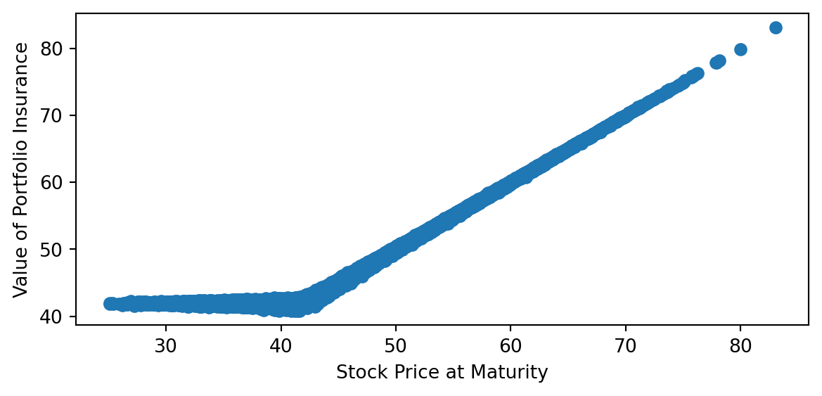
Ninety fifth percentile
0.31540269503348367
Notice that the largest hedging errors occur when the option expires near the money. This is beacuse the change in the delta around this point (Gamma) is large. Decreasing the hedging frequency will generally lead to larger hedging errors.
9.6 Delta-Gamma Hedging
To attempt to improve the performance of a discretely rebalanced delta hedge, one can use another option to create a portfolio that is both delta and gamma neutral. Being delta neutral means hedged as in the previous section—the portfolio value has no exposure to changes in the underlying asset price. In other words, it means that the derivative of the portfolio value with respect to the price of the underlying (the portfolio delta) is zero. Being gamma neutral means that the delta of the portfolio has no exposure to changes in the underlying price, which is equivalent to the second derivative of the portfolio value with respect to the price of the underlying (the portfolio gamma) being zero. If the delta truly did not change, then there would be no need to rebalance continuously, and hence no hedging error introduced by only adjusting the portfolio at discrete times rather than continuously. However, there is certainly no guarantee that a discretely rebalanced delta/gamma hedge will perform better than a discretely rebalanced delta hedge.
A delta/gamma hedge can be constructed as follows. Suppose we have written (shorted) a call option and we want to hedge both the delta and gamma using the underlying asset and another option, for example, another call option with a different strike. In practice, one would want to use a liquid option for this purpose, which typically means that the strike of the option will be near the current value of the underlying (i.e., the option used to hedge would be approximately at the money).
Let \(\delta\) and \(\Gamma\) denote the delta and gamma of the written option and let \(\delta^*\) and \(\Gamma^*\) denote the delta and gamma of the option used to hedge. Consider holding \(a\) shares of the stock and \(b\) units of the option used to hedge in conjunction with the short option. The delta of the stock is one (\(\mathrm{d} S/\mathrm{d} S = 1\)), so to obtain a zero portfolio delta we need
\[ 0 = - \delta + a + b\delta^*. \qquad(9.1)\]
The gamma of the stock is zero (\(\mathrm{d}^2 S/\mathrm{d} S^2 = d\,1/\mathrm{d} S = 0\)), so to obtain a zero portfolio gamma we need
\[ 0 = - \Gamma + b\Gamma^*\;. \qquad(9.2)\]
Equation Equation 9.2 shows that we should hold enough of the second option to neutralize the gamma of the option we have shorted; i.e., \[ b= \frac{\Gamma}{\Gamma^*} \] Equation Equation 9.1 shows that we should use the stock to delta hedge the portfolio of options; i.e., \[ a=\delta - \frac{\Gamma}{\Gamma^*}\delta^*\;. \]
9.7 Implied Volatilities
While all other Black-Scholes inputs are observable, volatility must be estimated. Given an option’s market price, we can invert the Black-Scholes formula to find the implied volatility—the \(\sigma\) that produces the observed price.
Implied volatilities serve several purposes:
- Price quotes: Options are often quoted in terms of implied volatility
- Relative value: Comparing implied volatilities helps identify expensive or cheap options
- Market views: Implied volatilities reflect market expectations of future volatility
The Volatility Smile
If the Black-Scholes model were perfect, all options with the same maturity would have the same implied volatility. In practice, plotting implied volatility against strike typically shows:
- Higher implied volatilities for low strikes (out-of-the-money puts)
- Lower implied volatilities near the at-the-money strike
- Slightly increasing implied volatilities for high strikes
This “volatility smile” or “smirk” indicates that market prices reflect: - Fat tails: Higher probability of extreme moves than lognormal - Negative skewness: Larger probability of extreme downward moves
The smile has been particularly pronounced for equity index options since the 1987 crash, suggesting market participants price in crash risk.
9.8 Exercises
Digital Options and Building Blocks
Exercise 9.1 Consider a cash digital option that pays $1 when \(S_T > K\) and a share digital that pays \(S_T\) when \(S_T > K\). Using Black-Scholes parameters \(S_0 = 100\), \(K = 105\), \(r = 5\%\), \(q = 2\%\), \(\sigma = 20\%\), \(T = 0.25\).
- Calculate the analytical values of both digital options using the formulas from the chapter
- Verify your results using Monte Carlo simulation with 100,000 paths
- Show that a call option can be decomposed as: \(C = S_0 N(d_1) e^{-qT} - K N(d_2) e^{-rT}\)
- Implement this decomposition and verify it matches the standard Black-Scholes formula
Exercise 9.2 The delta of a cash digital option that pays $1 when \(S_T > K\) is \[\Delta_{\text{digital}} = \frac{e^{-rT} n(d_2)}{\sigma S \sqrt{T}}\,,\]
where \(n(\cdot)\) is the standard normal density.
- Plot this delta against stock price for \(S \in [80, 120]\) with the parameters from the previous exercise
- Compare the magnitude of digital delta to call option delta near the strike
- Explain why delta hedging a short digital position near expiration and near the strike is problematic
- What happens to the digital delta as time to expiration approaches zero?
Exercise 9.3 The following two questions can be answered in two ways.
- What is the vaule of a derivative security that pays \(\mathbf{1}_{\{S_T <K\}}\)?
- What is the value of a derivative security that pays $ S_T _{{S_T <K}}$?
Change of Numeraire and Girsanov’s Theorem
Exercise 9.4 Using simulation, verify the change of numeraire formulas for digital options:
- Under the risk-neutral measure, simulate \(S_T\) following \(dS/S = (r-q)dt + \sigma dB^R\)
- Under the stock numeraire measure, simulate \(S_T\) following \(dS/S = (r-q+\sigma^2)dt + \sigma dB^S\)
- Calculate \(\mathbb{E}^R[e^{-rT} \mathbf{1}_{\{S_T > K\}}]\) and \(S_0 \mathbb{E}^S[\mathbf{1}_{\{S_T > K\}}/S_T]\)
- Verify both give the same digital option value up to simulation error
- Use 50,000 simulation paths and report the standard errors
Exercise 9.5 Verify the exponential martingale property in Girsanov’s Theorem. With \(\kappa = (\mu - r)/\sigma\):
- Simulate paths of \(Z_t = \exp(-\frac{1}{2}\kappa^2 t - \kappa B_t)\) where \(B_t\) is standard Brownian motion
- Verify that \(\mathbb{E}[Z_T] = 1\) for various values of \(T\)
- Show that \(Z_t S_t/R_t\) is a martingale under the original measure
- Compare the distribution of \(B_t + \kappa t\) to standard Brownian motion under the new measure
Black-Scholes Formula and Properties
Exercise 9.6 Implement the complete Black-Scholes formula with all Greeks:
- Create a Python class
BlackScholesOptionthat calculates price, delta, gamma, theta, vega, and rho - Include both calls and puts with proper dividend yield handling
- Verify put-call parity: \(C - P = S_0 e^{-qT} - K e^{-rT}\)
- Test your implementation against the interactive Black-Scholes explorer values
Exercise 9.7 Analyze the limiting behavior of the Black-Scholes formula:
- Show that as \(T \to 0\), the call value approaches \(\max(S_0 - K, 0)\)
- Show that as \(\sigma \to 0\), the formula approaches the deterministic payoff present value
- What happens to call and put values as \(\sigma \to \infty\)? Explain intuitively.
- Analyze the behavior as \(r \to 0\) and as \(r \to \infty\)
Exercise 9.8 Using the interactive Black-Scholes explorer or your own implementation:
- For an at-the-money option, plot call value against volatility for \(\sigma \in [0.1, 1.0]\)
- Repeat for options that are 10% in-the-money and 10% out-of-the-money
- For which moneyness is the option price most sensitive to volatility changes?
- Explain this pattern in terms of the option’s probability of finishing in-the-money
Greeks and Risk Management
Exercise 9.9 Create comprehensive plots of the Greeks using the interactive Greeks explorer as reference:
- Plot delta, gamma, theta, vega, and rho against stock price for an at-the-money option
- Repeat for different times to expiration: 1 month, 3 months, 6 months, 1 year
- Identify where gamma is maximized and explain why this matters for hedging
- Show how theta changes as expiration approaches and explain the time decay acceleration
Exercise 9.10 Consider delta and gamma hedging a short call option using the underlying and a put with the same strike and maturity:
- Derive the positions in stock and put needed for a delta-gamma neutral portfolio
- Show that this hedge never needs adjustment (relate to put-call parity)
- Implement this strategy and compare hedging errors to delta-only hedging
- What are the practical limitations of this “perfect” hedge?
The Fundamental PDE and Replication
Exercise 9.11 Show that the stock price and the boond price satisfy the fundamental PDE with the appropriate boundary condition.
Exercise 9.12 Show that the share digital and cash digital prices satisfy the fundamenatl PDE with the appropriate boundary condition.
Exercise 9.13 Use risk neutral valuation to find the value of a derivative security which pays \(\ln(S_T)\). Verify your value satisfies the fundamental PDE with the appropriate boundary condition. What is the replicating portfolio? Is this option harder to hedge than a standard option? Why or why not?
Exercise 9.14 Calculate the Greeks for exotic payoffs:
- For a derivative paying \(S_T^2\), find the value, delta, and gamma using risk-neutral valuation
- For a derivative paying \(\log(S_T)\), repeat the calculation
- Verify both satisfy the fundamental PDE: \(rV = \frac{\partial V}{\partial t} + (r-q)S\frac{\partial V}{\partial S} + \frac{1}{2}\sigma^2 S^2 \frac{\partial^2 V}{\partial S^2}\)
- Compare the hedging difficulty (gamma exposure) of these payoffs to standard options.
Exercise 9.15 Modify the code which simulates delta hedging to simulate replication of a cash digital option. Where do the largest errors tend to occur? Compare the hedging difficulty (gamma exposure) of these payoffs to standard options.
Exercise 9.16 Modify the code which simulates delta hedging to incur a transaction cost. One model has ask price \(1.01 S_t\) and and bid price share \(0.99 S_t\). Another model has ask price \(S_t +.005\) and bid price \(S_t - .005\). Try different rebalancing frequencies. What rebalancing frequency gives the best hedging? Where do the largest errors tend to occur?
Discrete Hedging and Practical Implementation
Exercise 9.17 Extend the discrete hedging simulation from the chapter:
- Compare hedging errors for different rebalancing frequencies: daily, weekly, monthly
- Analyze how hedging errors scale with volatility and time to expiration
- Study the impact of transaction costs: assume 0.1% bid-ask spread on each rebalance
- Find the optimal rebalancing frequency that minimizes total cost (hedging error + transaction costs)
Exercise 9.18 Analyze the gamma scalping strategy:
- Show that a delta-hedged short option position has P&L approximately equal to \(-\frac{1}{2}\Gamma(\Delta S)^2\)
- Simulate this P&L for different realized volatilities vs. implied volatility
- Demonstrate that selling options when implied volatility > realized volatility is profitable
- Account for the theta decay and show the complete P&L attribution
Implied Volatility and Market Practice
Exercise 9.19 Implement an implied volatility calculator:
- Use numerical methods (bisection or Newton-Raphson) to invert the Black-Scholes formula
- Test with market-like option prices and verify convergence
- Handle edge cases: very deep ITM/OTM options, very short/long expirations
- Compare computational efficiency of different numerical methods
Delta-Gamma Hedging
Exercise 9.20 Consider delta and gamma hedging a short call option, using the underlying and a put with the same strike and maturity as the call. Calculate the position in the underlying and the put that you should take, using the analysis in the Delta-Gamma Hedging section. Will you ever need to adjust this hedge? Relate your result to put-call parity.
Exercise 9.21 Modify the discrete delta hedging simulation to compute percentiles of gains and losses for an investor who writes a call option and constructs a delta and gamma hedge using the underlying asset and another call option. Include the exercise price of the call option used to hedge as an input, and assume it has the same time to maturity as the option that is written.
Hint: In each period, the updated cash position can be calculated as:
Cash = exp(r*dt)*Cash + a*S*(exp(q*dt)-1) - (Newa-a)*NewS - (Newb-b)*PriceHedgewhere a denotes the number of shares of the stock held, b denotes the number of units held of the option that is used for hedging, and PriceHedge denotes the price of the option used for hedging (computed from the Black-Scholes formula each period). This expression embodies the interest earned (paid) on the cash position, the dividends received on the shares of stock and the cash inflows (outflows) from adjusting the hedge. At the final date, the value of the hedge is:
exp(r*dt)*Cash + a*S*(exp(q*dt)-1) + a*NewS + b*max(NewS-KHedge,0)and the value of the overall portfolio is the value of the hedge less max(NewS-KWritten,0), where KHedge denotes the strike price of the option used to hedge and KWritten denotes the strike of the option that was written.
9.9 Summary
The Black-Scholes model combines the theoretical foundations of arbitrage pricing with practical implementation:
- Change of numeraire: Digital options under different measures give the formula
- Replication: Delta hedging shows how to replicate option payoffs
- Fundamental PDE: All Europena style derivatives satisfy the same partial differential equation with diffrent boundary conditions.
- Greeks: Sensitivities guide risk management and hedging
- Market practice: Implied volatilities reveal market expectations and model limitations
The model’s elegance lies in showing that, under its assumptions, options can be perfectly hedged through dynamic trading. While real markets violate these assumptions, the Black-Scholes framework remains the foundation for understanding option pricing and hedging.
See Karatzas and Shreve (1991).↩︎
If numsims = 11 and pct =0.1, the percentile function returns the second lowest element in the series. The logic is that 10% of the numbers, excluding the number returned, are below the number returned—i.e., 1 out of the other 10 are below—and 90% of the others are above. In particular, if pct = 0.5, the percentile function returns the median. When necessary, the function interpolates; for example, if numsims = 10 and pct=0.1, then the number returned is an interpolation between the lowest and second lowest numbers.↩︎
The implementation uses vectorized calculations to improve performance (typically much faster than pure Python loops).↩︎